Transient Thermal Conduction Example

Introduction

This tutorial was created using ANSYS 7.0 to solve a simple transient conduction problem. Special thanks to Jesse Arnold for the analytical solution shown at the end of the tutorial.

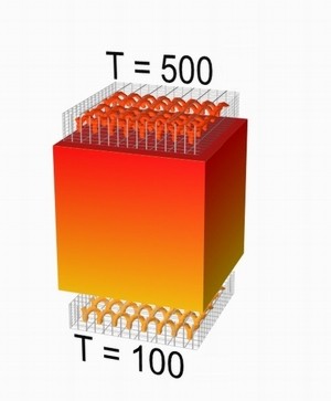
The example is constrained as shown in the following figure. Thermal conductivity (k) of the material is 5 W/m*K and the block is assumed to be infinitely long. Also, the density of the material is 920 kg/m^3 and the specific heat capacity (c) is 2.040 kJ/kg*K.

It is beneficial if the Thermal-Conduction tutorial is completed first to compare with this solution.

Preprocessing: Defining the Problem

Give example a Title

Utility Menu > File > Change Title...
/Title,Transient Thermal Conduction

Open preprocessor menu

ANSYS Main Menu > Preprocessor
/PREP7
Create geometry

Preprocessor > Modeling > Create > Areas > Rectangle > By 2 Corners
X=0, Y=0, Width=1, Height=1
BLC4,0,0,1,1
　Define the Type of Element

Preprocessor > Element Type > Add/Edit/Delete... > click 'Add' > Select Thermal Mass Solid, Quad 4Node 55
ET,1,PLANE55

For this example, we will use PLANE55 (Thermal Solid, Quad 4node 55). This element has 4 nodes and a single DOF (temperature) at each node. PLANE55 can only be used for 2 dimensional steady-state or transient thermal analysis.
Element Material Properties

Preprocessor > Material Props > Material Models > Thermal > Conductivity > Isotropic > KXX = 5 (Thermal conductivity)
MP,KXX,1,10

Preprocessor > Material Props > Material Models > Thermal > Specific Heat > C = 2.04
MP,C,1,2.04

Preprocessor > Material Props > Material Models > Thermal > Density > DENS = 920
MP,DENS,1,920
- Mesh Size
Preprocessor > Meshing > Size Cntrls > ManualSize > Areas > All Areas > 0.05
AESIZE,ALL,0.05
Mesh

Preprocessor > Meshing > Mesh > Areas > Free > Pick All
AMESH,ALL

At this point, the model should look like the following:

Solution Phase: Assigning Loads and Solving

Define Analysis Type

Solution > Analysis Type > New Analysis > Transient
ANTYPE,4

The window shown below will pop up. We will use the defaults, so click OK.

Set Solution Controls

Solution > Analysis Type > Sol'n Controls

The following window will pop up.

A) Set Time at end of loadstep to 300 and Automatic time stepping to ON.
B) Set Number of substeps to 20, Max no. of substeps to 100, Min no. of substeps to 20.
C) Set the Frequency to Write every substep.

Click on the NonLinear tab at the top and fill it in as shown

D) Set Line search to ON .
E) Set the Maximum number of iterations to 100.

For a complete description of what these options do, refer to the help file. Basically, the time at the end of the load step is how long the transient analysis will run and the number of substeps defines how the load is broken up. By writing the data at every step, you can create animations over time and the other options help the problem converge quickly.

Apply Constraints

For thermal problems, constraints can be in the form of Temperature, Heat Flow, Convection, Heat Flux, Heat Generation, or Radiation. In this example, 2 sides of the block have fixed temperatures and the other two are insulated.
　

Solution > Define Loads > Apply
Note that all of the -Structural- options cannot be selected. This is due to the type of element (PLANE55) selected.
　

Thermal > Temperature > On Nodes
　

Click the Box option (shown below) and draw a box around the nodes on the top line and then click OK.

The following window will appear:

　

Fill the window in as shown to constrain the top to a constant temperature of 500 K
　

Using the same method, constrain the bottom line to a constant value of 100 K
Orange triangles in the graphics window indicate the temperature contraints.

Apply Initial Conditions

　
Solution > Define Loads > Apply > Initial Condit'n > Define > Pick All
Fill in the IC window as follows to set the initial temperature of the material to 100 K:

Solve the System

　
Solution > Solve > Current LS
SOLVE

Postprocessing: Viewing the Results

Results Using ANSYS
　

Plot Temperature

General Postproc > Plot Results > Contour Plot > Nodal Solu ... > DOF solution, Temperature TEMP

Animate Results Over Time
　

First, specify the contour range.
Utility Menu > PlotCtrls > Style > Contours > Uniform Contours...
Fill in the window as shown, with 8 contours, user specified, from 100 to 500.

　

Then animate the data.
Utility Menu > PlotCtrls > Animate > Over Time...
Fill in the following window as shown (20 frames, 0 - 300 Time Range, Auto contour scaling OFF, DOF solution > TEMP)

You can see how the temperature rises over the area over time. The heat flows from the higher temperature to the lower temperature constraints as expected. Also, you can see how it reaches equilibrium when the time reaches approximately 200 seconds. Shown below are analytical and ANSYS generated temperature vs time curves for the center of the block. As can be seen, the curves are practically identical, thus the validity of the ANSYS simulation has been proven.

Analytical Solution

ANSYS Generated Solution

Time History Postprocessing: Viewing the Results

Creating the Temperature vs. Time Graph
　
　

Select: Main Menu > TimeHist Postpro. The following window should open automatically.

If it does not open automatically, select Main Menu > TimeHist Postpro > Variable Viewer

　

Click the add button in the upper left corner of the window to add a variable.
　

Select Nodal Solution > DOF Solution > Temperature (as shown below) and click OK. Pick the center node on the mesh, node 261, and click OK in the 'Node for Data' window.

　

The Time History Variables window should now look like this:

Graph Results over Time
　

Ensure TEMP_2 in the Time History Variables window is highlighted.
　

Click the graphing button in the Time History Variables window.
　

The labels on the plot are not updated by ANSYS, so you must change them manually. Select Utility Menu > Plot Ctrls > Style > Graphs > Modify Axes and re-label the X and Y-axis appropriately.

Note how this plot does not exactly match the plot shown above. This is because the solution has not completely converged. To cause the solution to converge, one of two things can be done: decrease the mesh size or increase the number of substeps used in the transient analysis. From experience, reducing the mesh size will do little in this case, as the mesh is adequate to capture the response. Instead, increasing the number of substeps from say 20 to 300, will cause the solution to converge. This will greatly increase the computational time required though, which is why only 20 substeps are used in this tutorial. Twenty substeps gives an adequate and quick approximation of the solution.

Command File Mode of Solution

The above example was solved using a mixture of the Graphical User Interface (or GUI) and the command language interface of ANSYS. This problem has also been solved using the ANSYS command language interface that you may want to browse. Open the .HTML version, copy and paste the code into Notepad or a similar text editor and save it to your computer. Now go to 'File > Read input from...' and select the file. A .PDF version is also available for printing.