Thermal - Mixed Boundary Example (Conduction/Convection/Insulated)

Introduction

This tutorial was created using ANSYS 7.0 to solve simple thermal examples. Analysis of a simple conduction as well a mixed conduction/convection/insulation problem will be demonstrated.

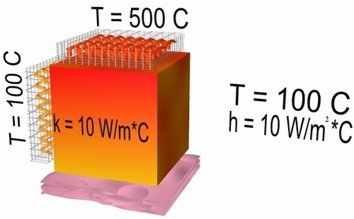
The Mixed Convection/Conduction/Insulated Boundary Conditions Example is constrained as shown in the following figure (Note that the section is assumed to be infinitely long):

Preprocessing: Defining the Problem

1. Give example a Title
2. Open preprocessor menu

ANSYS Main Menu > Preprocessor

/PREP7

• Create geometry

Preprocessor > Modeling > Create > Areas > Rectangle > By 2 Corners > X=0, Y=0, Width=1, Height=1
BLC4,0,0,1,1

• Define the Type of Element

  Preprocessor > Element Type > Add/Edit/Delete... > click 'Add' > Select Thermal Mass Solid, Quad 4Node 55
  ET,1,PLANE55　

  As in the conduction example, we will use PLANE55 (Thermal Solid, Quad 4node 55). This element has 4 nodes and a single DOF (temperature) at each node. PLANE55 can only be used for 2 dimensional steady-state or transient thermal analysis.

• Element Material Properties

  Preprocessor > Material Props > Material Models > Thermal > Conductivity > Isotropic > KXX = 10
  MP,KXX,1,10

  This will specify a thermal conductivity of 10 W/m*C.

  Mesh Size

  Preprocessor > Meshing > Size Cntrls > ManualSize > Areas > All Areas > 0.05
  AESIZE,ALL,0.05

• Mesh

　Preprocessor > Meshing > Mesh > Areas > Free > Pick All
AMESH,ALL

Solution Phase: Assigning Loads and Solving

1. Define Analysis Type

   　

2. Solution > Analysis Type > New Analysis > Steady-State
   ANTYPE,0

Apply Conduction Constraints 

In this example, all 2 sides of the block have fixed temperatures, while convection occurs on the other 2 sides.

	Solution > Define Loads > Apply > Thermal > Temperature > On Lines
	Select the top line of the block and constrain it to a constant value of 500 C
	Using the same method, constrain the left side of the block to a constant value of 100 C

Apply Convection Boundary Conditions

	Solution > Define Loads > Apply > Thermal > Convection > On Lines
	Select the right side of the block. The following window will appear:

Fill in the window as shown. This will specify a convection of 10 W/m2*C and an ambient temperature of 100 degrees Celcius. Note that VALJ and VAL2J have been left blank. This is because we have uniform convection across the line.

Apply Insulated Boundary Conditions

	Solution > Define Loads > Apply > Thermal > Convection > On Lines
	Select the bottom of the block.
	Enter a constant Film coefficient (VALI) of 0. This will eliminate convection through the side, thereby modeling an insulated wall. Note: you do not need to enter a Bulk (or ambient) temperature

You should obtain the following:

Solve the System

Solution > Solve > Current LS
SOLVE

Postprocessing: Viewing the Results

Results Using ANSYS

Plot Temperature

General Postproc > Plot Results > Contour Plot > Nodal Solu ... > DOF solution, Temperature TEMP

Command File Mode of Solution  

The above example was solved using a mixture of the Graphical User Interface (or GUI) and the command language interface of ANSYS. This problem has also been solved using the ANSYS command language interface that you may want to browse. Open the .HTML version, copy and paste the code into Notepad or a similar text editor and save it to your computer. Now go to 'File > Read input from...' and select the file. A .PDF version is also available for printing.

網內資料: